A paper posted to arXiv this month drops a finding that should make every team running a neural anomaly detector pause and check their baselines. A simple linear autoregressive model, solved in closed form with ordinary least squares regression, matches or outperforms 21 leading deep learning detectors on time series anomaly detection across five benchmark datasets. The method requires orders of magnitude less compute. If you are paying GPU bills to flag anomalies in metrics, logs, or sensor streams, the fanciest model in the room may not be the best one for the job.
The OLS baseline scored 0.9399 mean F1 across all five datasets, second only to KANAD at 0.9559, while winning on two stricter evaluation metrics outright.
Linear baselines strike back
The paper, titled "Strong Linear Baselines Strike Back," evaluates OLS regression against 21 baselines on five diverse anomaly detection datasets covering both univariate and multivariate time series. Three evaluation metrics are used: F1, E-F-5 (existence-level F1 with tolerance 5), and B-F-5 (buffered F1 with tolerance 5). The tolerance-based metrics are stricter about when an anomaly counts as correctly detected, requiring the prediction to land within a window of the true anomaly segment.
OLS achieved the lowest average rank across all three metrics combined. It posted the highest mean E-F-5 score of 0.6963 and the highest mean B-F-5 score of 0.7335 among all 22 methods tested. On plain F1, it scored 0.9399, placing second behind KANAD's 0.9559. The gap on F1 between first and second is 0.016, a difference that falls within the noise range for most production monitoring systems.
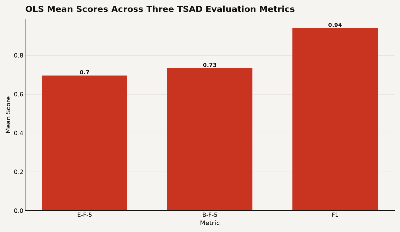
The chart above shows OLS's mean scores across the three evaluation metrics. The plain F1 score looks strong at 0.9399, but the E-F-5 and B-F-5 scores reveal where the real separation between methods lives. These tolerance-based metrics reward precise localization of anomalies, and OLS dominates them.
A separate study published around the same time reinforces the finding from a different angle. Researchers comparing PCA, a linear dimensionality reduction technique dating back decades, against OmniAnomaly, a stochastic VAE-based recurrent neural network, on the Server Machine Dataset found that PCA achieved performance comparable to OmniAnomaly and occasionally surpassed it, particularly when point-adjustment was not applied. The study ran 100 repetitions across 28 machines and concluded that performance differences were driven primarily by thresholding strategy and evaluation protocol, not by model architecture.
A third study, also from DLR, compared six methods (three classical, three deep) on the UCR Anomaly Archive's 250 univariate time series. The classical methods generally outperformed the deep learning methods across a range of anomaly types. The deep methods tested included autoencoders, graph augmented normalizing flows, and transformer-based TranAD.
The theory behind the century-old method
The theoretical contribution of the paper provides the explanation. The authors prove that a linear autoregressive model with OLS estimation is equivalent to estimating a finite-history Gaussian process conditional density. In practical terms, the linear model captures any anomaly that manifests as a deviation from the expected conditional distribution of the next observation given recent history. Spike anomalies, level shifts, and variance changes all fall in this category, which covers the majority of patterns in current benchmarks.
Deep learning models theoretically capture more complex temporal dependencies and nonlinear relationships. The problem is that current benchmarks may not contain anomalies complex enough to require those capabilities. The authors explicitly call for new benchmarks with richer temporal structures that can isolate where deep learning provides genuine advantages. Until those benchmarks exist, the performance gap between linear and deep remains untested in the regimes where deep models are supposed to excel.
This echoes a pattern visible across ML evaluation. When a compressed 4-bit LLM outperforms its full-precision parent, the benchmark failed to stress the capability that full precision was designed to protect. The same dynamic applies here. The benchmarks are valid for what they test, but they may be too simple to differentiate linear from nonlinear approaches.
The evaluation methodology compounds the problem. The PCA-vs-OmniAnomaly study identifies three factors that inflate deep model scores in published results: the anomaly score model itself, the threshold selection procedure, and the evaluation protocol. Point-adjustment, a common practice that credits a detection if any point in a contiguous anomaly segment is flagged, can inflate F1 scores substantially. When the researchers disabled point-adjustment and evaluated at point level, the deep model's advantage disappeared on most machines.
Anomaly detection pipelines, reconsidered
If you are building or maintaining a time series anomaly detection system, the practical implications are concrete:
- Start with OLS before reaching for deep learning. Fit a linear autoregressive model on your historical data. It trains in seconds on a CPU, needs no GPU, and gives you a deployable baseline today. If it catches the anomalies you care about, you have saved yourself a model training pipeline, a GPU budget, and weeks of hyperparameter tuning.
- Audit your thresholding protocol. The choice of threshold can swing F1 scores more than the choice of model. A global statistic threshold paired with point-adjustment can inflate scores by hiding false positives. Run your evaluation at point level, without adjustment, to see true detection performance.
- Report per-entity metrics, not just averages. The PCA study found that aggregated F1 scores mask substantial variability across machines. An average F1 of 0.85 across 28 servers can hide individual machines at 0.40. Identify the entities where your detector underperforms and investigate why.
- Reconsider your compute spend. If a linear model achieves comparable accuracy at orders of magnitude lower cost, the GPU hours you are spending on deep inference may be buying architectural fashion rather than detection quality.
- Use stricter evaluation metrics. Plain F1 can be misleading. The E-F-5 and B-F-5 metrics, which apply tolerance windows, exposed larger gaps between methods. If your internal evaluation uses only F1, you are missing the signal that separates precise detectors from lucky ones.
It depends on your data
The answer depends on your data, and the paper offers guidance. On the Server Machine Dataset, specific machines identified as 1-7 and 2-8 performed substantially better with OmniAnomaly than with PCA. Those entities likely have nonlinear correlations and temporal dependencies that linear methods cannot capture. If your data has those characteristics, a deep model earns its keep.
The decision framework is straightforward. Deploy OLS first and measure its per-entity performance. Identify the entities where it underperforms. Then evaluate whether a deep model specifically improves detection on those entities, under the same thresholding and evaluation protocol. If it does, use it for those entities and keep OLS for the rest. If it does not, you have eliminated a GPU cluster from your infrastructure bill.
The authors also make a broader point about research norms. They argue that future TSAD papers should consistently include strong linear baselines. A new deep detector that fails to beat OLS has only shown the benchmark is too easy. The field needs benchmarks with richer temporal structures to pinpoint genuine deep learning advantages, and until those exist, claims of deep learning superiority rest on untested assumptions.
The cost of skipping the baseline
The finding that OLS matches or beats 21 deep detectors is a tax audit on a subfield that has spent years optimizing for architectural novelty over empirical rigor. Every team that deployed a deep anomaly detector without first checking whether a linear model would suffice has been paying a compute tax for accuracy they could have gotten for free. The fix is cheap, the evidence is strong, and the baseline has been available for a century.
Sources
- arXiv - Strong Linear Baselines Strike Back: Closed-Form Linear Models as Gaussian Process Conditional Density Estimators for TSAD
- arXiv - Systematic comparison of PCA and OmniAnomaly on the Server Machine Dataset
- DLR Applied Sciences - Is It Worth It? Comparing Six Deep and Classical Methods for Unsupervised Anomaly Detection in Time Series
- Reddit r/MachineLearning - Original discussion thread