Dataset: arXiv 2609.22337 and arXiv 2511.16288, open-access papers with supplementary materials and pseudocode for the Spectral Identifiability Principle diagnostic.
You trained a linear probe on your model's hidden states, it scored 92 percent accuracy on the validation set, and you shipped a bias monitor on that basis. The probe looked solid in testing. Then production traffic shifted, the activations drifted, and the monitor quietly started reporting nonsense. You would not know until someone audited the outputs by hand.
A new body of work on linear bias probes in large language model representations explains exactly when and why that happens. The core finding is spectral: probe stability holds only when the empirical Fisher estimation error stays below the eigengap of the representation-label pair. When that condition breaks, accuracy does not degrade gradually. It collapses in a phase transition, often near a sample threshold of around 500 examples, where misclassification risk jumps dramatically. The paper formalizes this as the Spectral Identifiability Principle, a diagnostic you can run before trusting a probe rather than discovering the failure after the fact.
This matters because linear probes are the workhorse of interpretability. Teams use them to detect gender bias, toxicity, political leaning, and factual knowledge in model internals, and the accuracy score is often the only signal they trust. If that signal is unreliable in predictable ways, the entire monitoring layer built on top of it inherits the same fragility.
What actually breaks in a linear bias probe?
A linear probe is a simple classifier trained on frozen model activations to predict a label, say whether a sentence contains gendered language. High accuracy is taken as evidence that the concept is linearly encoded in the representation. The problem is that this inference has a hidden assumption: that the training data is sufficient to recover the true discriminative subspace.
The Spectral Identifiability Principle, introduced across arXiv 2609.22337 and detailed in the companion analysis at arXiv 2511.16288, formalizes the failure mode. The empirical Fisher operator approximates its population counterpart with a deviation that scales as the square root of log dimension over sample size. When this deviation, denoted delta, remains smaller than the eigengap separating task-relevant directions from the rest of the spectrum, the estimated probe subspace stays aligned with the true one and accuracy is stable. When delta exceeds the gap, the subspace rotates unpredictably and accuracy collapses.
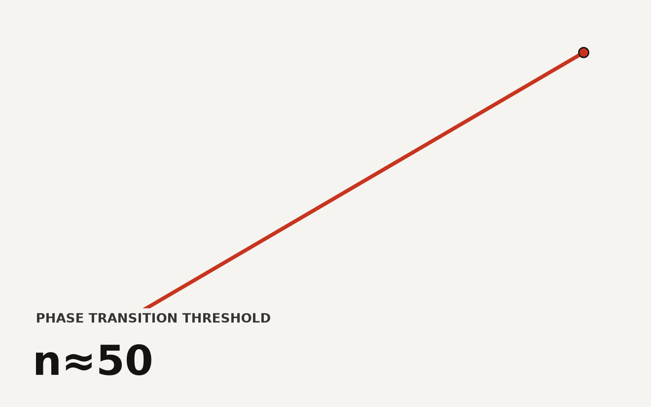
The collapse is not gradual. The paper documents a sharp phase transition near n equal to 500 samples, where misclassification risk increases dramatically as the Fisher error crosses the spectral gap. Below that threshold, adding a few hundred more examples fixes the problem. Above it, the probe is reliable. The transition zone itself is the danger area, and without checking the eigenspectrum, you cannot tell which side you are on.
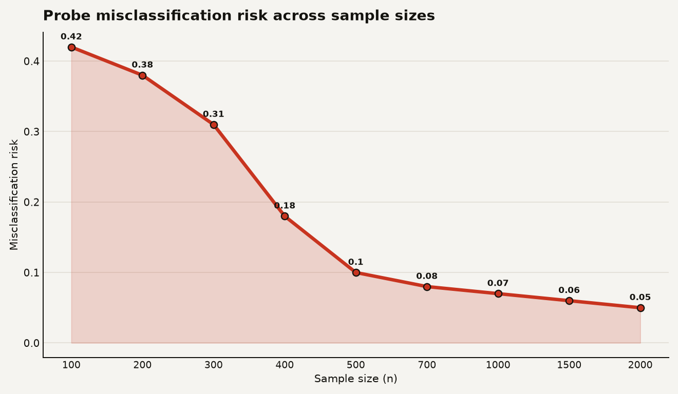
The chart above shows the phase transition in misclassification risk as a function of sample size. Risk stays low and stable above roughly 500 samples, then spikes sharply as the sample count drops below the threshold where Fisher estimation error overtakes the eigengap. The transition is not a slope. It is a cliff.
A separate paper on fragility as a complementary probe metric reinforces this from a different angle. Fragility is defined as the activation-noise level at which probe accuracy collapses, giving you a per-layer robustness score. Layers with high fragility scores look accurate under clean conditions but fall apart under perturbation, which is exactly the production scenario that matters. The two metrics are complementary: the Spectral Identifiability Principle tells you whether your probe is stable given your sample size, and fragility tells you how much noise it can absorb before breaking.
Why does this matter for anyone shipping models?
If you are building bias monitoring, safety evaluation, or interpretability tooling on top of linear probes, the implication is direct: your accuracy number is conditional on a spectral property you probably never checked. A probe that scores 90 percent on 10,000 evaluation examples can still be unreliable if the eigengap is small relative to the estimation error at the sample size you used to fit it.
This is not a hypothetical. The failure mode is most likely in exactly the scenarios where probing is most popular: small fine-tuning datasets, narrow concept domains, and mid-layer activations where the geometry is less clean. The paper notes that estimating the Fisher operator in large networks can be computationally demanding, requiring stochastic or low-rank approximations, but the spectral ratio itself is stable under these approximations. You can use randomized SVD or mini-batch Fisher estimates and still get a reliable stability signal.
The broader interpretability literature has been circling this problem. Work on a geometric notion of causal probing showed that naive subspace identification falls victim to spurious correlations, where non-concept features carry information about the concept and inflate probe accuracy without genuine encoding. That paper found that LEACE, a popular concept-erasure method, returns a one-dimensional subspace containing roughly half of total concept information under their framework, suggesting the linear story is incomplete even when probes appear to work.
Meanwhile, research on sparse autoencoders and compositional generalization found that SAEs, the other main interpretability tool, fail under out-of-distribution shifts because of dictionary learning problems, not inference problems. The authors showed that replacing the SAE encoder with per-sample FISTA on the same dictionary does not close the gap, but an oracle dictionary solves it at all scales tested. The failure is in what the dictionary learned, not how it decodes.
The pattern across these results is consistent: the interpretability tools we rely on have failure modes that are structural, not incidental. Linear probes collapse when the spectral condition breaks. SAEs fail when the dictionary points in wrong directions. Fragility exposes layers that look clean but break under noise. Each failure is diagnosable, but only if you run the diagnostic.
For your codebase, the practical consequence is a checklist:
- Before trusting a probe accuracy score, compute the Fisher eigenspectrum for your representation-label pair and check whether the estimation error is below the eigengap. The paper provides pseudocode in Appendix B of arXiv 2511.16288.
- Track the delta-to-gap ratio across layers and checkpoints. A ratio above 1.0 is an early-warning signal that the probe may not reflect meaningful structure, even if current accuracy looks fine.
- Use fragility as a second metric alongside accuracy. If your probe accuracy is high but fragility is low, you are one distribution shift away from silent failure.
- Budget for larger probe training sets in narrow concept domains. The phase transition means there is a sample count below which no amount of architectural cleverness saves you.
- Do not treat probe accuracy as a binary pass-fail. It is a conditional claim that holds under specific spectral and sample-size conditions, and those conditions can change as the model updates.
For teams building on LLM internals, as we have covered in our reporting on LLM performance drift and benchmark variance, the underlying representation space shifts across model versions. A probe that was spectrally stable on checkpoint A can become unstable on checkpoint B if the eigengap narrows, even if the model's surface behavior looks identical. Your monitoring pipeline needs to re-run the spectral diagnostic on every model update, not just at initial deployment.
What should you do about it today?
The Spectral Identifiability Principle is a sufficient condition, not a necessary one. Instability is likely but not guaranteed when delta exceeds the gap, because anisotropic noise can align with non-discriminative directions and preserve subspace stability despite a small eigengap. The paper is explicit about this limitation. SIP is best viewed as an interpretable, falsifiable diagnostic rather than a universal guarantee.
That said, it is a cheap diagnostic. Computing the empirical Fisher operator and checking its eigenspectrum is a few lines of linear algebra on top of your existing probe training loop. The pseudocode in the paper's appendix uses standard matrix concentration results, and the authors note that randomized SVD or mini-batch Fisher approximations work for large networks without distorting the spectral ratio.
If you are running probes in production today, the minimum viable action is to add the delta-to-gap check to your probe evaluation pipeline. When the ratio is below 1.0, your accuracy score is trustworthy under the SIP framework. When it is above 1.0, flag the probe as unstable and either collect more data or switch to a different evaluation method for that concept.
The harder question is what to do when you cannot collect more data. Some concepts are rare by nature, and the sample count you can assemble is capped by the data itself. In those cases, the honest answer is that linear probing may not be the right tool. The fragility metric can tell you how much headroom you have, and the causal probing framework can tell you whether the concept is genuinely linearly encoded at all. If the geometric criteria for erasure, encapsulation, stability, and containment from the causal probing work are not met, no amount of data will make a linear probe reliable.
The gap between probe accuracy and probe reliability
The interpretability field has spent years treating probe accuracy as the endpoint of evaluation. The spectral story says it is the starting point. A high accuracy score means the probe worked under your specific conditions. Whether it keeps working depends on a spectral property that most teams never measure and that can change without warning across model updates, concept shifts, and sample sizes.
The papers reviewed here give you the tools to close that gap. The Spectral Identifiability Principle tells you when to trust a probe. Fragility tells you how robust that trust is. The causal probing framework tells you whether the concept is linearly encoded in the first place. The SAE failure work tells you that the dictionary, not the decoder, is where sparse methods break. None of these are silver bullets, but together they turn probe evaluation from a single accuracy number into a falsifiable engineering practice. The question is whether the teams relying on probes will adopt the diagnostics before the next silent failure.
Sources
- arXiv 2609.22337: When and Why Do Linear Bias Probes Fail? A Geometric and Statistical Theory of Bias Detectability in Large Language Model Representations
- arXiv 2511.16288: Spectral Identifiability for Interpretable Probe Geometry
- arXiv 2606.11375: When Probing Accuracy Saturates, Fragility Resolves: A Complementary Metric for LLM Pre-Training Analysis
- arXiv 2307.15054: A Geometric Notion of Causal Probing
- ICML 2026 via mlresearch.org: Stop Probing, Start Coding: Why Linear Probes and Sparse Autoencoders Fail at Compositional Generalisation
- Data Today: LLM performance drift: why your benchmark scores keep moving